▸  Personal Project

Portfolio
Allocation Model

A self-directed attempt to understand how allocators think about risk - built from scratch in Excel, VBA, and Python to explore four portfolio construction methodologies and the mechanics behind them.

30
Max Assets
4
Methods
GJR-GARCH
Vol Model
3yr
Price History

Four ways to think
about risk

The model dynamically adapts to any portfolio of up to 30 public equities and computes optimal weights under four distinct allocation philosophies - from naïve equal-weighting to fully optimised risk parity.

EW

Equal Weight

Equal capital to every security. The simplest benchmark - no assumptions about risk or correlation.

IV

Inverse Volatility

Weights inversely proportional to each asset's GARCH-estimated conditional volatility. Lower-risk names receive higher allocation.

ERC

Equal Risk Contribution

True risk parity. Every asset contributes equally to total portfolio variance - requires full covariance matrix and Python optimisation.

MinVol

Minimum Volatility

Minimises total portfolio variance subject to weight constraints. Naturally concentrates in the lowest-vol, least-correlated names.

Input to output
in four automated steps

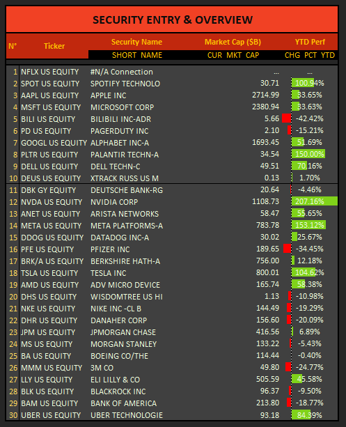
Step 01 - Security Entry

Define the universe

Enter Bloomberg tickers for up to 30 equities. The sheet uses BDP and BDH functions to auto-populate security names, live market capitalisations, and YTD performance in real time.

Bloomberg BDP / BDH Live market data Up to 30 assets
Security Entry worksheet

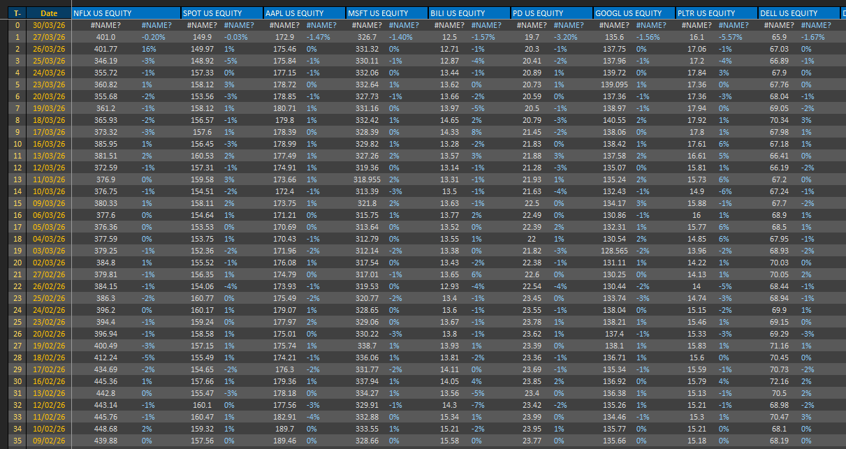
Step 02 - Price Data

Pull 3 years of history

Bloomberg fetches daily closing prices for each security going back 750 trading days. Daily returns are calculated alongside - these are the raw inputs that feed every downstream calculation.

BDH historical data ~750 observations Daily log returns
PX Data worksheet

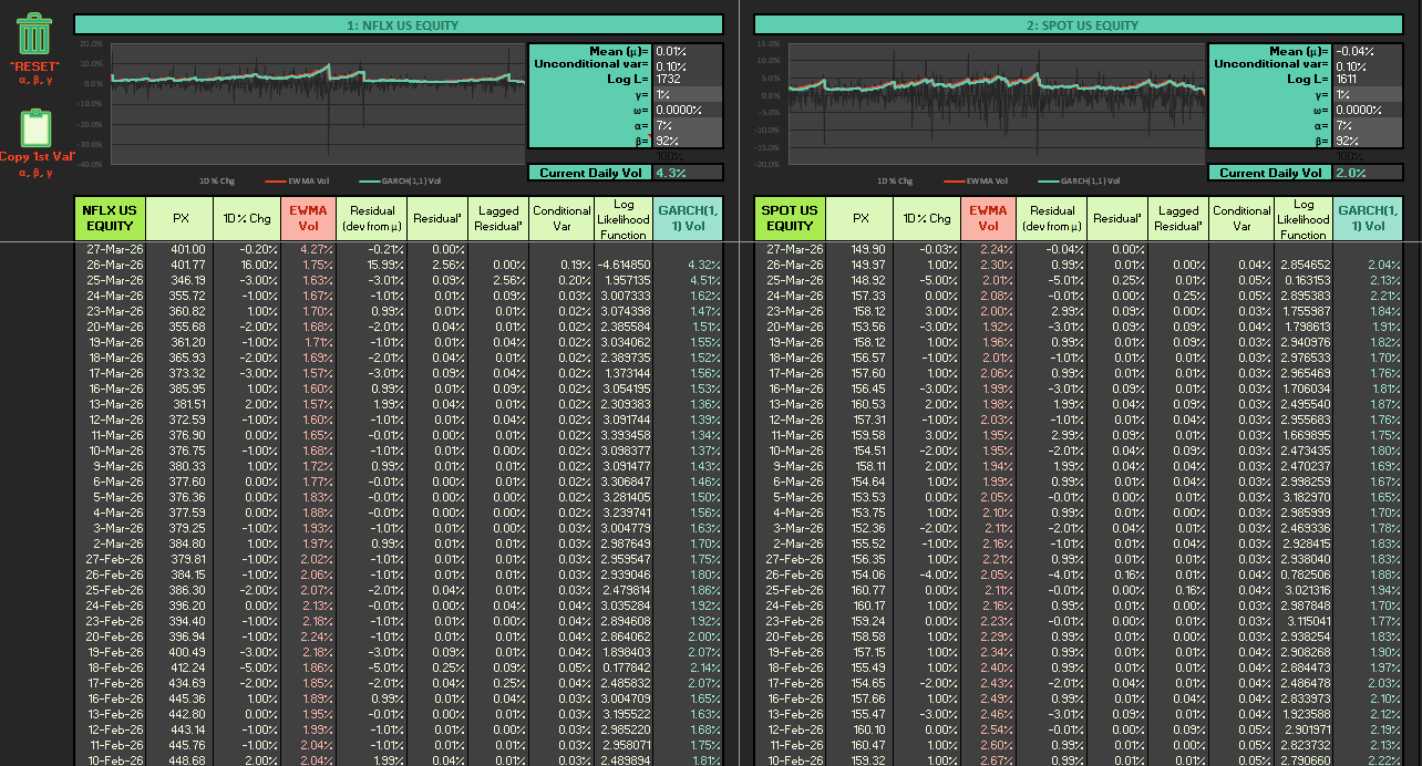
Step 03 - GARCH Volatility

Estimate dynamic volatility

A GJR-GARCH(1,1) model estimates conditional volatility for each security using 3 years of daily returns. Parameters α, β, and γ are optimised per asset by maximising the log-likelihood function via the Excel Solver.

GJR-GARCH(1,1) Max log-likelihood Per-asset calibration
GARCH volatility worksheet

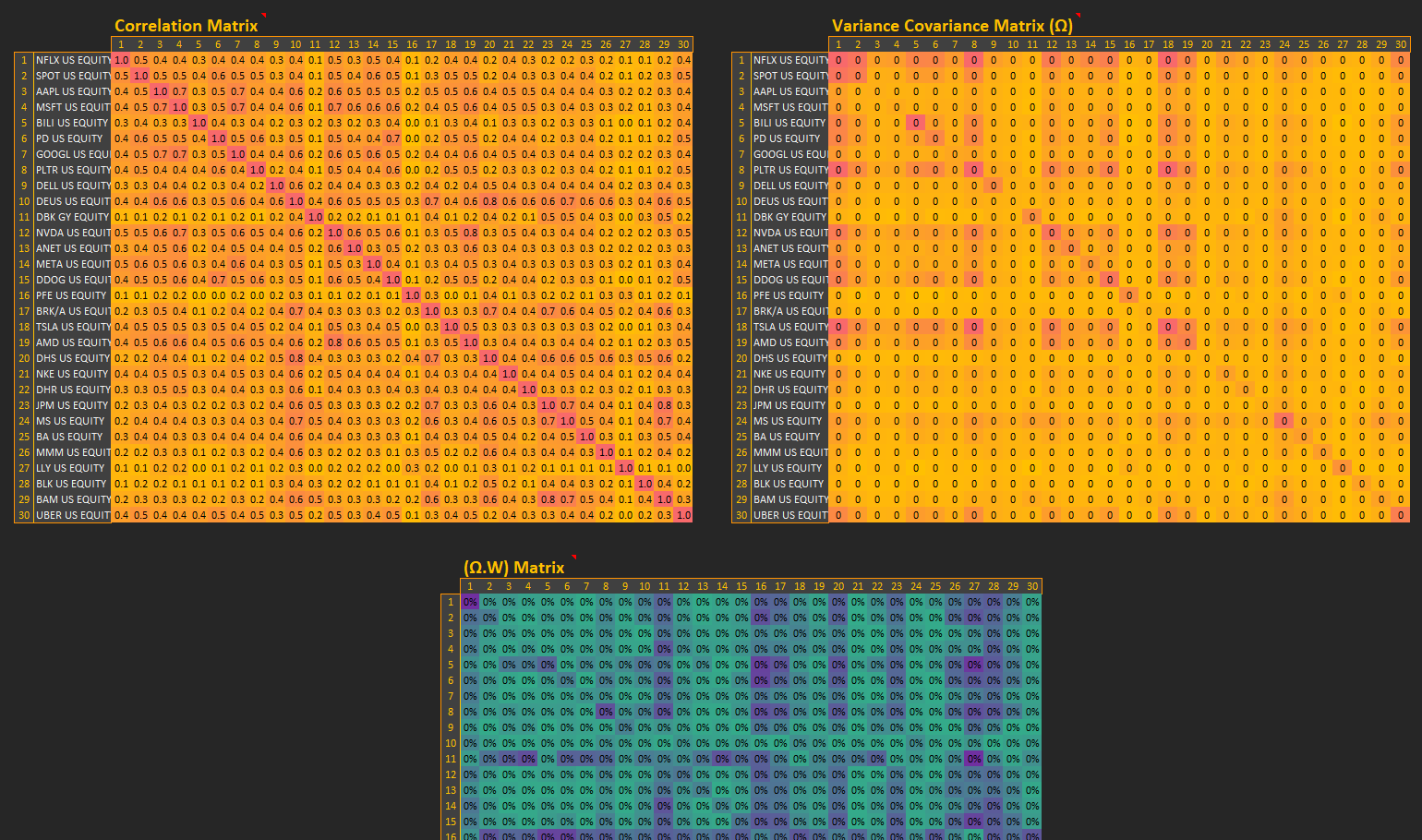
Step 04 - Matrix Construction

Build the covariance structure

Three matrices are computed: the correlation matrix, the variance-covariance matrix (Ω), and the Ω × Weights matrix. All are dynamically linked and update whenever the allocation method or underlying weights change.

Correlation matrix Var-Covar (Ω) Dynamic linking
Matrixes worksheet

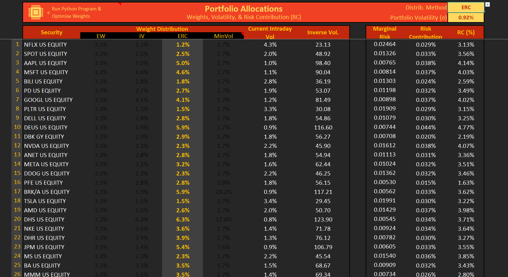
Step 05 - Portfolio Output

Optimised weights, instantly

Select the desired method from the DistMeth dropdown. EW and IV weights recalculate instantly. ERC and MinVol trigger standalone Python solvers - bundled as compiled executables, so no Python install is needed on the recipient machine.

ERC_Solver.exe MinVol_Solver.exe VBA macro trigger No Python required
Portfolio output worksheet

Under the hood

Two ideas sit at the core of the model: a time-varying estimate of each asset's risk, and an allocation rule that does something sensible with it.

Volatility - GJR-GARCH(1,1)

Why not just use a rolling standard deviation?

Historical vol treats every past return equally. GARCH assumes volatility is persistent - a big shock today makes tomorrow riskier - and lets recent observations matter more. The GJR variant adds an asymmetric term to capture the leverage effect: bad news (negative returns) tends to spike vol more than equivalent good news.

$$\omega^2_t = \omega + \alpha\,\varepsilon^2_{t-1} + \beta\,\omega^2_{t-1} + \gamma\,\mathbf{1}_{t-1}\,\varepsilon^2_{t-1}$$

where $\mathbf{1}_{t-1} = 1$ if $\varepsilon_{t-1} < 0$ (leverage indicator)

$\omega$ Long-run variance floor - keeps $\omega^2$ strictly positive
$\alpha$ ARCH term - sensitivity of variance to last period's shock
$\beta$ GARCH term - persistence of yesterday's variance estimate
$\gamma$ Asymmetry term - extra weight on negative return shocks

$\alpha + \beta + \gamma/2 < 1$ is the stationarity condition. Parameters are calibrated per asset by maximising the log-likelihood over 3 years of daily returns using the Excel Solver.

Allocation - Risk Parity

What does it mean to "equalise risk"?

Portfolio volatility is not just a weighted average of individual vols - it depends on how assets co-move. Given a weight vector $\mathbf{w}$ and variance-covariance matrix $\boldsymbol{\Omega}$, portfolio volatility is:

$$\omega_p = \sqrt{\mathbf{w}^\top \boldsymbol{\Omega}\,\mathbf{w}}$$

The risk contribution $\text{RC}_i$ of asset $i$ is its marginal contribution to $\omega_p$, scaled by its weight:

$$\text{RC}_i = \frac{w_i \cdot (\boldsymbol{\Omega}\mathbf{w})_i}{\omega_p}$$

By Euler's theorem, $\sum_i \text{RC}_i = \omega_p$. The three allocation methods each define a different target for these contributions:

IV $w_i \propto 1/\omega_i$ - ignores correlations, fast to compute
ERC $\text{RC}_i = \text{RC}_j \;\forall\, i,j$ - true risk parity, requires numerical optimisation
MinVol $\min_{\mathbf{w}}\;\mathbf{w}^\top\boldsymbol{\Omega}\mathbf{w}$ s.t. $\textstyle\sum w_i=1,\; w_i\geq 0$

Try the model

Full Package (.zip)

Includes the Excel workbook, both solver executables, and a README. Requires Microsoft Excel with macros enabled and Bloomberg Terminal access for live data.

~160 MB · assembled in your browser on click